Category: AI Trends

There is a moment in every voice AI demo where something clicks. The agent responds quickly, the rhythm feels right, and the conversation moves forward the way a real conversation does. Then the same team ships to production, and the first thing users say is: “Why does it pause so long?”

That pause is not a model problem. Benchmarks published in late 2025 from 30-plus independent platform tests show that most voice agents in production still clock in at 800ms to two full seconds end-to-end.

The reason is pipeline compounding. Every stage in the voice agent stack adds time, and those stages run sequentially. Each handoff adds overhead. Endpointing waits for silence. Audio buffers in chunks. The LLM waits for a complete transcript. TTS waits for a complete LLM response. By the time sound reaches the user’s ear, a dozen small decisions have each added 50 to 200 milliseconds, and the total has long since crossed the threshold where conversations feel natural.

This post pulls that apart layer by layer. What are the actual numbers at each stage? Where do teams waste the most time? What does a well-architected low-latency pipeline look like in 2026? And what does it mean specifically for teams building in India, where geography adds an unavoidable physics tax on top of

The 300ms Rule and Why It Is Not Just a User Experience Concern

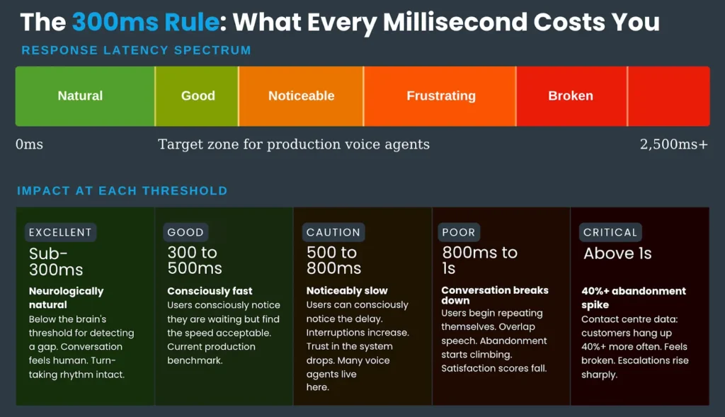
Research consistently puts the natural human conversational gap at 100 to 400 milliseconds. This is not a UX preference, it is a neurological baseline. Beyond 300ms, users may not consciously register a delay. Beyond 500ms, they can consciously notice it. Beyond one second, the conversation starts to feel broken, users may speak again assuming the agent did not hear them, interruptions multiply, and abandonment rates spike. Abandonment rates climb more than 40% when latency exceeds one second.

Latency is a paralinguistic signal. When a voice agent pauses, users read that pause as meaning something uncertain, failure, machine-ness. The rhythm of a conversation can shape how its content is received.

There is also an operational cost here that is separate from user experience. Longer interactions cost more to run. More pauses can mean more false turn detections, more correction cycles, more agent time per call. A team handling 50,000 calls a day saw clean average latency metrics, but churn and complaints stayed high because their P99 latency was spiking, affecting a small but vocal slice of users consistently.

This is the case for tracking P95 and P99 metrics, not just averages. A 400ms average with 2-second P99 spikes means users are abandoning calls even though the dashboard looks fine.

Where the Time Actually Goes: The Pipeline Breakdown

The standard cascaded voice agent pipeline has six sequential stages, each contributing to the total latency. This is what Introl’s voice AI infrastructure guide published in January 2026 summarises as the core equation: STT + LLM + TTS + network + processing equals roughly 1,000ms for a typical deployment, even when individual components are performing well.

Pipeline Stage	Typical Range	Optimised Target	Main Lever
Audio buffering + endpointing	250 to 600ms	20 to 80ms	Streaming chunks + smart endpointing model
Network upload (audio)	20 to 100ms	20 to 40ms	Edge proximity, WebSocket
STT processing (cloud)	100 to 500ms	Sub-100ms (streaming)	Streaming Conformer model, regional endpoint
STT processing (on-device)	250 to 520ms typical	Sub-50ms	CPU-first model, no network hop
LLM inference	350ms to 1,000ms+	150 to 300ms	Model size, 4-bit quantisation, streaming
TTS synthesis (first audio)	100 to 400ms	40 to 95ms	Streaming TTS, fire on first sentence
Network download (audio)	20 to 100ms	20 to 40ms	Edge proximity, WebSocket
Total (unoptimised)	800ms to 2,000ms	300 to 500ms	Architecture across all layers

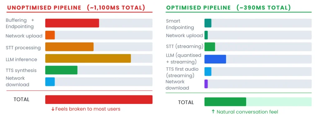
A few things stand out. First, audio buffering and endpointing are responsible for far more latency than most teams expect. Traditional silence-based endpointing defaults to a 500ms wait window before deciding a user has finished speaking. That 500ms alone exceeds the entire optimised target for some pipeline stages. Second, the LLM is almost always the single largest contributor once you have sorted the front end. Third, the gap between typical and optimised is not a technology gap. These optimised numbers are achievable today with components that are already in production.

Stage One: Audio Buffering and Endpointing

Most teams skip past this because it feels like plumbing rather than AI. That is a mistake. Endpointing is where many pipelines lose 300 to 600ms before any model has seen a single byte of audio.

Traditional end-of-turn detection works on silence. The system waits for the user to stop speaking, then waits a further 500ms silence window to confirm the turn is over, then passes the full buffer to STT. Most silence-based endpointing defaults sit around 500ms, and reducing that threshold is risky because natural pauses inside a sentence can look like end-of-turn events. The result is a system that either cuts people off mid-sentence or adds 500ms of avoidable latency on every turn.

Smart endpointing replaces silence detection with a trained model that reads richer signals: prosody, semantic completion, vocal pattern. Models must be built specifically for this task: detecting when a speaker stops talking as fast as possible. Because it should understand context rather than just silence, it can use tighter timing thresholds without the false-positive problem. Faster endpointing can directly reduce the time before the STT model even begins.

Stage Two: STT Processing and the Streaming vs Batch Divide

This is where most latency discussions start, but it is actually step two of the problem. STT architecture is the difference between a pipeline that can hit sub-100ms and one that cannot.

Batch STT waits for a complete audio buffer before transcription begins. Streaming STT transcribes continuously as audio arrives, returning partial outputs in real time using Connectionist Temporal Classification (CTC)-style alignment-free decoding approaches that produce frame-synchronous output without waiting for the full utterance. The difference in time-to-first-token is large: batch systems typically take 300 to 500ms, streaming systems deliver first tokens in under 100ms in production.

Conformer-based architectures have become the standard for low-latency streaming ASR. They combine convolutional layers for local acoustic patterns efficiently with self-attention for longer-range dependencies. A 2025 arXiv paper on telecom voice pipelines using a Conformer-CTC architecture achieved real-time factors below 0.2 on GPU, meaning the model processes audio faster than it arrives.

Stage Three: LLM Inference- The Biggest Budget Item

Once you have solved endpointing and STT, the LLM is almost always the place where latency budgets collapse. Standard LLM inference on a large model takes 350ms to well over one second depending on context length, model size, and available compute. For a pipeline already at 150ms STT, a 700ms LLM call produces a total latency of 850ms before TTS has even started.

AssemblyAI’s engineering team made a point worth quoting directly: reducing TTS latency from 150ms to 100ms sounds meaningful, but if your LLM takes 2,000ms, you have improved total latency by 2.5%. The optimisation effort should go where the time actually is.

There are four well-established approaches to this, all of them practical in 2026:

1. Stream LLM output to TTS from the first token. Do not wait for a complete response before starting synthesis. Fire the TTS call as soon as the first sentence is available, then continue streaming. This parallelises two expensive stages and reduces perceived latency dramatically because the user begins hearing the response while the model is still generating.
2. Apply 4-bit quantisation. A 2025 arXiv paper on telecom voice pipelines found that 4-bit quantisation achieves up to 40% latency reduction while preserving over 95% of original model performance. For most voice agent tasks, the accuracy tradeoff is imperceptible.
3. Right-size the model. A 7B or 13B parameter model processes a turn significantly faster than a 70B model, and for most constrained voice agent tasks, intent classification, FAQ response, appointment booking, a well-prompted small model performs a large general model on both speed and cost.
4. Pre-load retrieval context. If your agent uses RAG, load the domain documents before the call begins rather than retrieving at inference time. For constrained domains, cache common response patterns entirely to bypass inference for known queries.

Stage Four: TTS Synthesis and the Last Hundred Milliseconds

TTS has improved faster than any other component in the voice AI stack over the last 18 months. Most tools are genuinely fast, and the architecture for squeezing more out of TTS is straightforward: stream.

Start synthesis the moment the first sentence of LLM output arrives. Play that audio to the user while the model generates the second sentence. Continue streaming. The user experiences near-zero TTS latency because audio starts before synthesis is complete. Hamming AI’s latency guide notes that streaming TTS can reduce perceived latency to under 100ms for the user even when full synthesis takes 300ms, because what matters is time-to-first-byte, not time-to-complete-audio.

One nuance the Twilio team identified is worth keeping: a faster system can feel subjectively slower if the voice is less expressive. Prosody and naturalness affect perceived latency even when the actual milliseconds are the same. For customer-facing applications, test voice quality alongside speed metrics. A 10ms slower TTS that sounds noticeably more human often wins on user satisfaction even though it loses on the dashboard.

The Network Layer: The Variable Nobody Optimises

Model and pipeline choices get most of the engineering attention. Network architecture gets almost none of it, and for teams building in India, this is where the most avoidable latency lives.

Geography can create latency that no model optimisation can overcome. A round trip from Mumbai to a US-East endpoint adds 180 to 250ms of network latency purely from physics, before any processing. On a multi-turn conversation, that compounds to multiple seconds of cumulative overhead. The simplest fix is also the most impactful: use a regional endpoint.

Architecture Choice	Latency Impact	When to Use
REST API (per request)	+50 to 100ms per turn	Batch workflows only, never for real-time voice
WebSocket (persistent)	Near-zero connection overhead	All real-time voice applications
Cloud, US endpoint (from India)	+180 to 250ms per turn	When data can leave India and regional is unavailable
Cloud, India regional endpoint	+20 to 50ms	Default for India deployments
On-device / on-premise	Sub-100ms (no network)	Regulated industries, air-gap, DPDPB compliance

For Indian enterprise deployments, this is a critical calculation. The DPDPB and sector-specific regulations in BFSI and healthcare create data residency requirements that make US-endpoint cloud routing genuinely problematic, not just slow. On-premise or edge deployment of the STT layer solves both problems simultaneously; it eliminates the network latency penalty and satisfies data residency without any quality compromise, because modern CPU-first models run at production-grade accuracy without cloud infrastructure.

Putting It Together: A Realistic Latency Budget

Good latency engineering starts from a budget. Here is a realistic target breakdown for a sub-500ms voice agent pipeline using current technology:

Component	Target Budget	How to Hit It
Audio buffering	20 to 40ms	20ms streaming chunks, WebSocket from the start
Smart endpointing	50 to 80ms	Dedicated endpointing model, not silence detection
STT (cloud, regional)	80 to 120ms	Streaming Conformer CTC, India regional endpoint
STT (on-device)	Sub-50ms	CPU-first model, zero network overhead
LLM inference	150 to 250ms	7B to 13B quantised model, stream from first token
TTS first audio	40 to 95ms	Streaming TTS, fire on first LLM sentence
Network round-trip	20 to 40ms	Regional endpoint or on-device, WebSocket
Total (cloud path)	360 to 525ms	Well-architected cascaded pipeline
Total (on-device STT)	280 to 415ms	On-device STT + cloud LLM + streaming TTS

A few things stand out in this budget. The LLM is still the single largest item, which is why right-sizing it matters more than shaving milliseconds off TTS. On-device STT produces lower total latency than cloud STT in most India deployments, because eliminating zooms of network overhead outweighs any processing difference. The gap between the optimised total and the typical production total, 300 to 500ms versus 800 to 2,000ms, is not explained by model capability. It is explained by architecture decisions at every stage.

The teams winning on latency are not using faster models. They are using better architecture; streaming at every layer, right-sized LLMs, regional or on-device inference, and WebSocket connections throughout.

Latency Is an Architecture Problem

The teams shipping sub-500ms voice agents in 2026 are not using secret models or experimental infrastructure. They are making better architecture decisions at every layer: streaming audio from the start, using smart endpointing instead of silence windows, right-sizing their LLMs, streaming TTS from the first token, and placing inference as close to users as data residency requirements allow.

Sub-100ms STT is achievable today. The gap between that and a total pipeline below 500ms is a series of well-understood engineering choices, not unsolved problems. The reason most production agents are still at 800ms to two seconds is that teams optimise components in isolation rather than profiling the pipeline as a whole and finding the actual bottleneck.

For teams building in India, for BFSI, healthcare, contact centres, regional language applications, there is an additional dimension. Geography is a physics problem, not a software problem. On-device CPU-first STT resolves it cleanly: no network round-trip, full data residency compliance, and latency performance that often beats cloud from a standing start. The architecture that satisfies compliance requirements turns out to also produce the fastest pipelines.

Build the pipeline right from the start. Latency is much easier to architect in than to retrofit.

References

• Assemblyai.com. (2025). The 300ms rule: Why latency makes or breaks voice AI applications. [online] Available at: https://www.assemblyai.com/blog/low-latency-voice-ai [Accessed 11 Mar. 2026].
• Digital Minds BPO (2024). 30+ Eye-Opening Call Center Statistics and Metrics You Must Know in 2025. [online] Outsourcing Philippines | Digital Minds BPO. Available at: https://digitalmindsbpo.com/blog/call-center-statistics.
• Ethiraj, V., David, A., Menon, S. and Vijay, D. (2025). Toward Low-Latency End-to-End Voice Agents for Telecommunications Using Streaming ASR, Quantized LLMs, and Real-Time TTS. [online] arXiv.org. Available at: https://arxiv.org/abs/2508.04721 [Accessed 11 Mar. 2026].
• Introl.com (2026). Welcome To Zscaler Directory Authentication. [online] Available at: https://introl.com/blog/voice-ai-infrastructure-real-time-speech-agents-asr-tts-guide-2025 [Accessed 11 Mar. 2026].
• Xu, M. (2026). Voice AI Latency Benchmarks: What Agencies Need to Know in 2026. [online] Trillet.ai. Available at: https://www.trillet.ai/blogs/voice-ai-latency-benchmarks [Accessed 11 Mar. 2026].
• You.com (2026). You.com | What Is P99 Latency? Why It Matters and How to Improve It. [online] Available at: https://you.com/resources/what-is-p99-latency [Accessed 11 Mar. 2026].

The last generation of enterprise software made a trillion dollars by digitizing the artifacts of work. Contracts went into DocuSign. Calls went into Gong. Customer conversations went into Salesforce transcripts.

The record was the thing that survived; the conversation that created it was discarded like scaffolding.

Voice is having its GPT-3 moment. Latency has collapsed. Interruption handling works. Emotional tone inference is real.

A new generation of voice AI companies is racing to deploy agents across every phone-heavy workflow in the enterprise: sales, support, collections, scheduling, healthcare intake, field service dispatch.

The pitch is compelling to replace or augment a $250 billion global call center industry with software that never sleeps and scales infinitely.

That pitch is right, but incomplete. The race to replace the call center agent misses the larger prize. It’s the equivalent of seeing the internet and building a better fax machine.

The real opportunity is not in automating the conversation. It’s in finally capturing what conversations contain: the signals, commitments, hesitations, and decisions that human workers have always processed in real time and immediately forgotten.

We call the accumulated structure formed by those captured signals a conversation graph: not a transcript archive, but a living record of intent, commitment, and decision stitched across interactions, entities, and time so that what a customer revealed in frustration six months ago is available context the next time they call.

What existing systems don’t capture from voice

Every enterprise has invested heavily in CRM, support tooling, and analytics. They record calls. They do post-call summaries. Some even run sentiment scoring. And yet the highest-signal channel in customer relationship management remains, paradoxically, the least understood.

The problem isn’t volume. It’s that voice carries information that doesn’t survive transcription, and that even when it does, the systems receiving that information were never designed to act on it:

Signal Type	What It Contains	What CRM Captures	What’s Lost
Paralinguistic cues	Hesitation, rising tone, pacing changes	Close to nothing	Intent signals, uncertainty
Soft commitments	“I’ll loop in our CFO by Thursday”	~50% of the time, in free text	Follow-up triggers, deal risk
Emotional trajectory	Escalating frustration across 3 calls	Each ticket routed fresh	Churn prediction, relationship health
Negotiation subtext	What’s meant vs. what’s said	Literal words only	True objection mapping

Paralinguistic signals that indicate intent.

The customer who says “that sounds fine” while their voice rises and slows is not convinced. The prospect who answers a qualifying question after a long pause is uncertain. These signals aren’t in the transcript. They’ve never been in any system. They lived in the rep’s gut and left when the rep did.

Commitments made in conversation but never logged.

“I’ll loop in our CFO by Thursday.” “We’d consider a longer term if pricing were flexible.” These soft commitments get mentioned in the post-call summary if the rep remembers. Half the time they don’t make it into the CRM. And when they do, there’s no system watching for whether they materialize or expire.

Emotional trajectory across interactions.

A customer who has called three times with escalating frustration is on a churn path that the ticket system doesn’t see, it routes each call fresh. No system connects the dots: this is the same person, this is the pattern, this is what previous agents promised, this is where the relationship is headed.

The delta between what’s said and what’s meant.

Enterprise sales, collections, and support are all, at their core, negotiation. What someone says in a negotiation is not what they mean. The experienced rep knows this. The CRM records the literal words.

This is what “never captured” means in the voice context. Not dirty data. Not siloed systems. The information was simply never treated as data in the first place. It passed through a human, was processed unconsciously, influenced a decision, and evaporated.

“Voice is the highest-bandwidth channel in the enterprise. It has also been, until now, the least legible one.”

The conversation graph is the enduring asset

When startups instrument the voice layer to capture not just transcripts but signals, hesitation patterns, commitment language, emotional inflection, question sequences, topic drift and connect those signals to entities and outcomes, they build something enterprises have never had: a queryable model of how spoken interaction actually drives decisions.

What does this look like in practice?

A renewal call surfaces that the primary contact has used phrases like “our team is evaluating options” three times in the last two quarters. The conversation graph links that signal to a historical pattern: accounts using that language 90 days pre-renewal churn at 3x the baseline.

The voice agent doesn’t just handle the renewal call. It enters it with a risk score, routes mid-call to a human when a commitment signal weakens, and writes a structured trace: not just “call completed” but “objection raised: pricing vs. ROI; contact tone shifted positive at minute 11; commitment to follow-up secured.”

The feedback loop is what makes this compound. Each call adds to the graph. The graph improves the next call. Outcomes, whether the commitment materialized, whether the account churned, whether the deal closed, flow back as labels. The model becomes genuinely predictive, not because it was trained on some generic dataset, but because it was trained on this company’s customers, in this industry, with this product.

This is the distinction that matters:

Rules tell an agent what to say when (“if the customer mentions a competitor, ask about switching costs”).

The conversation graph captures what actually happened: the moment hesitation appeared, the commitment that was made, the emotional arc that preceded churn, and why the agent escalated.

Over time, that graph becomes the real source of truth for voice autonomy—explaining not just what was said, but what it meant, and what happened next.

None of this requires full automation on day one. It starts with assisted calling: the agent listens, surfaces signals in real time, suggests responses, and records the trace. Over time, as patterns accumulate, more of the call can be handled autonomously. Even when a human is on the line, the graph keeps growing.

Why incumbents can’t build the conversation graph

Recording incumbents are in the analysis path, not the execution path.

Gong is exceptional at post-hoc insight: deal risk scores, topic trends, coaching recommendations. But Gong sees a call after it’s over, via an integration. It doesn’t sit in the live conversation. It can’t surface a signal mid-call, adjust the agent’s approach in real time, or write a decision trace at the moment of commitment. By the time data reaches Gong, the most important context of what was happening emotionally in the room is already degraded into a transcript.

CRM and CCaaS players prioritize current state.

Salesforce knows what the opportunity looks like today. It doesn’t know what was said in the call that moved it from Stage 2 to Stage 3, what hesitation was present but unresolved, or what the customer’s voice revealed that the rep didn’t write down. When a deal goes dark, the CRM shows the last activity. There’s no “the customer’s commitment language dropped sharply after we mentioned implementation timelines” in the activity log.

Cloud telephony and CCaaS vendors are infrastructure providers.

Amazon Connect, Twilio, Genesys—these companies win on scale, reliability, and integrations. Their motion is horizontal plumbing, not vertical intelligence. They will sell transcription and summaries as commodities. They will not build the feedback loops that make a specific company’s conversation graph proprietary and compounding.

The structural advantage belongs to startups that are natively in the voice execution path—that own the conversation, not just a record of it. Those startups can capture context at the moment it exists: not after the call, not via ETL, but while the words are being spoken.

Three paths for startups –

Some will own vertical depth before horizontal scale.

Healthcare, insurance, financial services—industries where every call is a compliance artifact and where a single phrase can constitute a commitment, a disclosure, or a violation. In these verticals, the conversation graph is not a nice-to-have. It’s the product. The company that builds the richest model of how conversations in healthcare intake actually unfold has a moat that generalist voice platforms can never replicate.

Some will build the intelligence layer under existing voice infrastructure.

Rather than owning the call, they sit beneath it—instrumenting CCaaS deployments, adding real-time signal capture without requiring a platform rip-and-replace. The motion is faster to enterprise because it doesn’t require a telephony migration. The defense is depth of the graph itself—proprietary models trained on years of labeled outcomes that no new entrant can replicate.

Some will create entirely new categories of voice-native workflows.

These companies identify processes that have never been digitized because they require the nuance of human conversation—and they make those processes run on software for the first time. Think clinical decision support via voice with a field nurse. Think collections that actually negotiate rather than read scripts.

Key signals for founders

Two signals apply across all three paths:

High call volume with low CRM hygiene.

If a company makes 10,000 calls a month and the CRM has clean data on 2,000 of them, that gap is significant. It’s not laziness, it’s the impossibility of capturing what voice contains in a structured data entry form. That gap is the market.

Outcome variance that isn’t explained by the script.

If two reps following the same playbook produce wildly different results, the difference is in what they hear and how they respond, not what they say. That unexplained variance is evidence of unconverted signal, and unconverted signal is the conversation graph’s raw material.

One signal points specifically to new system of record opportunities:

Functions that exist to interpret rather than execute.

The sales manager who listens to call recordings to understand why deals stall. The customer success leads who audits support calls before QBRs. The compliance officer who spot-checks for regulatory language. These roles exist because organizations have given up on getting that intelligence from their software. That’s a tell: the function that does interpretation manually is pointing at the next system of record.

Voice as a system of record, reimagined

The question isn’t whether voice AI companies will displace call centers—they will. The question is whether the winners are the ones who move the most calls through software, or the ones who build the richest understanding of what conversations contain.

Call volume is a commodity moat. The conversation graph is a compounding one. Every call makes it smarter. Every outcome labels it deeper. Every enterprise that builds on it becomes more dependent on it than on any telephony platform, because the graph represents something no one else has: a structured, predictive model of how this company’s customers actually communicate.

The last generation of enterprise software won by owning canonical data. The next generation wins by owning canonical understanding. In voice, that’s the conversation graph—and the startups building it today are laying the foundation for the next trillion-dollar category.

Picture this: A bank customer in Lucknow calls a contact centre voice bot and says “Mera account mein paisa credit nahi hua, please check karo.” The bot, built on a globally recognised ASR platform, returns a 40% word error rate. The word “credit” is transcribed as “cradle.” The word “paisa” is dropped entirely. The bot asks the customer to repeat themselves three times before escalating to a human agent.

This is not a hypothetical. It is what happens every day across millions of enterprise voice deployments in India. And it represents a market failure hiding in plain sight.

More than 900 million people are online in India today, the second-largest internet user base on earth. Among them, 98% consume content in Indic languages, with Tamil, Telugu, Hindi, and Malayalam dominating. Over half of urban internet users actively prefer regional language content over English. And yet the voice AI infrastructure that powers digital interactions, the IVR systems, the voice bots, the transcription engines, was built for a fundamentally different user: an English speaker with a standard accent, speaking in a quiet room.

The gap between who voice AI was built for and who actually uses it in India is the largest underserved opportunity in enterprise AI today. This post is our attempt to quantify it, explain why it is so technically hard, and lay out what building for it correctly actually requires.

The Scale of the Opportunity

India is not a monolingual market with a translation problem. It is a linguistically sovereign one. The Indian Constitution recognises 22 official languages. There are 30 languages with over a million native speakers each. There are more than 1,600 dialects.

When Jio disrupted mobile data pricing in 2016 and brought hundreds of millions of Indians online at near-zero cost, the majority of those new users were not English speakers. As Google’s then-VP for India Rajan Anandan noted at the time: “Almost every new user that is coming online, roughly nine out of 10, is not proficient in English.”

That wave has only accelerated. Rural India, which now accounts for 55% of India’s 886 million active internet users, is doubling its growth rate compared to urban areas. These users access the internet almost entirely via mobile, and they interact with it via their native language. The IAMAI’s Internet in India Report 2024 found that 57% even of urban internet users now prefer regional language content.

For voice AI, this creates an infrastructure imperative. Voice is the most natural interface for users who are not comfortable with text, for users navigating banking services, healthcare, government portals, and customer support in their first language. The contact centres, IVR systems, and voice bots being deployed to serve this population need to understand how these people actually speak. Most of them do not.

“Almost every new user that is coming online, roughly nine out of 10, is not proficient in English. So it is fair to say that almost all the growth of usage is coming from non-English users.”

– Rajan Anandan, former Google VP India

Language	Estimated Speakers (India)	Internet Users (est)	ASR Availability
Hindi	600M+	250M+	Moderate, accuracy degrades significantly on regional dialects
Bengali	100M+	50M+	Limited, few production-grade models
Marathi	95M+	45M+	Limited, near zero enterprise-grade coverage
Telugu	93M+	40M+	Limited, improving through IndicVoices datasets
Tamil	78M+	38M+	Moderate, more data available than other Dravidian languages
Gujarati	62M+	28M+	Very limited
Kannada	57M+	25M+	Limited
Odia, Punjabi, Malayalam	30-40M each	12-20M each	Sparse to none in production systems

Why Standard ASR Fails on Indic Languages

Understanding the Indic ASR gap requires understanding why it exists, and it is not simply a matter of collecting more training data. The challenges are structural, linguistic, and deeply intertwined.

1. The Code-Switching Problem

In real-world Indian speech, code-switching, the fluid alternation between two or more languages within a single conversation, or even a single sentence, is not an edge case. It is the norm.

A customer service call in Mumbai might involve a speaker who opens in Hindi, switches to English for a technical term, reverts to Hindi mid-sentence, and introduces a Marathi loanword in the same breath. This is not linguistic confusion, it is how multilingual Indians naturally communicate. The phenomenon is so common it has acquired colloquial names: Hinglish, Tanglish (Tamil-English), Benglish.

Standard ASR systems are fundamentally ill-equipped for this. A 2025 IEEE Access paper on code-switching ASR for Indo-Aryan languages found that “present systems struggle to perform adequately with code-switched data due to the complexity of phonetic structures and the lack of comprehensive, annotated speech corpora.” The paper notes that while multilingual ASR systems outperform monolingual models in code-switching scenarios, even state-of-the-art approaches show WERs of around 21–32% on Hindi-English and Bengali-English test sets, in controlled laboratory conditions.

2. Orthographic Variability

Unlike English, where spelling is largely standardised, many Indic languages have significant orthographic flexibility. Common suffixes in Hindi attach and split or merge in multiple legitimate ways. Code-mixed terms, English words rendered in Devanagari script, have no standardised transcription. Proper nouns, place names, and brand names follow no consistent romanisation convention.

A March 2026 preprint from arXiv introduced Orthographically-Informed Word Error Rate (OIWER)as a more accurate evaluation metric for Indic ASR precisely because standard WER systematically overpunishes models for legitimate orthographic variation. Their analysis found that WER exaggerates model performance gaps by an average of 6.3 points, meaning models are often performing better than their WER scores suggest, but also that the evaluation frameworks used to compare them are unreliable.

3. Data Scarcity

The most direct cause of Indic ASR underperformance is data. State-of-the-art English ASR models were trained on hundreds of thousands of hours of labelled audio. Comparable datasets for Indic languages are orders of magnitude smaller. The IndicVoices dataset from IIT Madras’ AI4Bharat, one of the most significant efforts to close this gap, covers 22 Indian languages, but at a fraction of the scale of English training corpora. Most Indic languages remain genuinely low-resource from an ML perspective.

The practical implication: a model fine-tuned on a few hundred hours of Hindi audio can degrade significantly when exposed to the dialect diversity of a real production environment, Bihar-accented Hindi, Rajasthani-accented Hindi, Hindi spoken by native Tamil speakers. Real-world audio, with its background noise, telephony compression, and spontaneous speech patterns, compounds the problem further.

4. The Evaluation Paradox

Even benchmarking Indic ASR accurately can be non-trivial. Standard benchmark datasets for India languages are often constructed from read-aloud speech, a speaker reads a prepared sentence into a studio microphone. This is categorically different from spontaneous, conversational speech in a contact centre, a telemedicine call, or a field agent interaction. Models that score well on benchmark WER might collapse in production.

This creates a market information failure: enterprise buyers compare STT vendors on benchmark scores that might not reflect real-world performance on their specific user base. The result is that deployments are built on models that sound plausible in a demo but can fail in production on the voices they are actually supposed to serve.

The Market No One Is Seriously Building For

Given the scale of the opportunity, the natural question is: why hasn’t this been solved already?

The major speech AI platforms are predominantly built by and for English-speaking markets. Their training infrastructure, data pipelines, evaluation frameworks, and product roadmaps are majorly English-centric. Multilingual support, where it exists, is typically implemented as a bolt-on: a Whisper-based model, a Google Chirp integration, or a transfer-learning approach that prioritises coverage (can we output something for 50 languages?) over accuracy (does it work in production for Hindi speakers from Bihar?).

The companies building voice AI today are solving for a user who looks like their engineering team. That user speaks English. The billion people coming online next do not.

The Indian AI ecosystem has produced some focused efforts. But building a foundation model for 22 official Indian languages, each with sub-variants, code-switching patterns, and domain-specific vocabulary (medical, legal, financial), at a production-grade accuracy, is an extraordinarily capital-intensive undertaking. It requires not just models but data pipelines, annotation infrastructure, evaluation frameworks, and domain-specific fine-tuning.

What a Real Solution Looks Like

Building production-grade Indic voice AI requires getting five things right simultaneously. Getting three of them right while failing on the other two might produce a system that works in the demo and fails in deployment.

1. Language-Native Training, Not Transfer Learning from English

The foundational error in most multilingual ASR approaches is using English acoustic models as a starting point and fine-tuning toward Indic languages. This works well enough for high-resource languages where you have thousands of training hours, it fails for genuinely low-resource Indic languages where the acoustic space, the phoneme inventory, and the prosodic patterns are structurally different from English.

A native model for Hindi is trained on Hindi audio from the ground up, with an acoustic front-end designed for the retroflex consonants, the aspirated plosives, and the vowel length distinctions that characterise Indo-Aryan languages. A fine-tuned English model might systematically mishandle these features regardless of how much Indic data you throw at it.

2. Code-Switching as a First-Class Requirement

Production Indic voice AI must treat code-switching as a primary use case, not an edge case to be handled by post-processing. This means training on code-switched corpora explicitly, implementing language identification at the utterance and sub-utterance level, and building acoustic models that can operate in a continuous multilingual space rather than switching between discrete language modes.

The architecture difference is significant. A system with discrete language detection followed by routing to monolingual models will always have a latency penalty and an accuracy degradation at language boundaries. A system trained natively on code-switched data builds the transition probability into the acoustic model itself.

3. Real-World Audio Conditioning

Enterprise deployments in India operate through telephony infrastructure, often 8kHz narrowband audio with compression artefacts, background noise, and channel distortion. Models trained on clean studio audio degrade severely in these conditions. Real-world audio conditioning means training on telephone-quality speech, building noise robustness into the acoustic front-end, and evaluating on data that reflects actual deployment conditions rather than benchmark datasets.

4. Domain Vocabulary Injection

A contact centre voice bot for an Indian bank needs to understand: “NEFT transfer,” “Aadhaar-linked account,” “NACH mandate,” “UPI ID.” A medical transcription system needs to handle drug names pronounced in the way Indian clinicians actually pronounce them, often blending English pharmacological terms with native pronunciation patterns. Domain vocabulary injection, the ability to add entities and terms to the recognition grammar without retraining the base model, is a production requirement, not a nice-to-have.

5. Deployment Flexibility

Enterprise buyers in India, particularly in BFSI, healthcare, and government, have stringent data residency requirements. Patient audio cannot leave a HIPAA-equivalent boundary. Bank customer calls cannot transit international infrastructure. Building voice AI that can be deployed on-premise, in a private cloud, or at the edge, with CPU-first inference that does not require GPU infrastructure, is a prerequisite for winning regulated enterprise deals, not a feature differentiation.

Requirement	Standard Global ASR	Purpose-Built Indic ASR
Code-switching accuracy	WER 30-45% on Hinglish	WER <10% with native code-switch training
Regional accent robustness	Degrades significantly	Trained on dialect-stratified corpora
Telephony audio quality	Requires clean audio	Conditioned on 8kHz narrowband speech
Domain vocabulary	Static vocabulary only	Dynamic vocabulary injection supported
Deployment model	Cloud-only	Cloud, on-premise, edge, air-gap
Data residency	Cloud provider dependent	Fully on-premise available
Language coverage	3-5 Indic languages (basic)	22+ Indic languages with dialect variants

The Industries Being Reshaped

The Indic voice AI opportunity is not uniform across sectors. Three verticals are in active transformation, and the quality of voice AI infrastructure will determine which companies emerge as winners.

BFSI: The Largest Contact Centre Surface in the World

Indian BFSI operates at a staggering scale. 10.62 billion digital transactions occurred per month in India in 2023, a figure that has only accelerated with UPI adoption. Behind these transactions sits a contact centre infrastructure serving hundreds of millions of customers, the majority of whom prefer and often require service in their regional language.

A bank deploying a voice bot for credit card queries must handle the full spectrum of Indian English accents, native Hindi, regional language requests, and the code-switched hybrids that define real customer speech. The difference between a voice bot that works and one that doesn’t is not brand or UI, it is the accuracy of the underlying ASR at the acoustic and linguistic level.

Healthcare: Where Accuracy Is Not Optional

Clinical documentation is one of the highest-stakes ASR applications: a transcription error that turns a drug dosage or contraindication into noise is not a bad customer experience, it is a patient safety issue. The Indian healthcare system serves over a billion people, increasingly through telemedicine platforms and AI-assisted clinical workflows. These systems require ASR that can handle doctor-patient conversations in Hindi, Tamil, Bengali, and their code-switched variants, with the accuracy, compliance posture, and latency characteristics that clinical workflows demand.

Vernacular Content and Media

India is the world’s largest consumer of mobile data, averaging 20 GB per month per user in 2025. The majority of that consumption is video and audio content in regional languages. Media production companies, OTT platforms, and content distributors need automated transcription, captioning, and subtitle generation at scale, in 20+ languages simultaneously, with turnaround times measured in minutes, not hours.

The Builders Who Show Up First Will Own the Infrastructure Layer

The history of technology infrastructure follows a consistent pattern: the engineers who solve the hard and technically demanding problem first, before the market fully understands it needs solving, end up owning the category.

Indic language voice AI is that problem today. It is technically hard. It requires years of investment in data infrastructure, acoustic modelling, and production hardening. It will not be solved by taking a model trained on English and adding a language detection header. And the market it unlocks, 900 million internet users, growing at double-digit rates, in the second-largest economy in the world, is not a niche.

The enterprises deploying voice AI in India right now are using infrastructure that might fail their users. They know it. They are looking for an alternative that actually works. The opportunity is not theoretical. The procurement cycles are live.

→ View Indic language benchmarks → Try Zero STT Indic free → Contact our India team

References

• •Arxiv.org. (2026). Towards Orthographically-Informed Evaluation of Speech Recognition Systems for Indian Languages. [online] Available at: https://arxiv.org/html/2603.00941v1 [Accessed 9 Mar. 2026].
• •Bureau, T.H. (2026). India now has 958 million active internet users; 57% of these are from rural areas. [online] The Hindu. Available at: https://www.thehindu.com/sci-tech/technology/india-now-has-958-million-active-internet-users-57-of-these-are-from-rural-areas/article70566646.ece
• •Grandviewresearch.com. (2026). India Conversational AI Market Size & Outlook, 2030. [online] Available at: https://www.grandviewresearch.com/horizon/outlook/conversational-ai-market/india [Accessed 9 Mar. 2026].
• •Hemant Palivela, Meera Narvekar, Asirvatham, D., Shashi Bhusan, Vinay Rishiwal and Agarwal, U. (2025). Code-Switching ASR for Low-Resource Indic Languages: A Hindi-Marathi Case Study. IEEE Access, pp.1–1. doi: https://doi.org/10.1109/access.2025.3527745
• •IAMAI (2023). Internet in India 2022. [online] Available at: https://www.iamai.in/sites/default/files/research/Internet%20in%20India%202022_Print%20version.pdf

Frequently Asked Questions

What is Indic language voice AI?

Indic language voice AI refers to speech recognition, voice synthesis, and voice agent systems designed specifically to handle the 22 official languages of India, including Hindi, Tamil, Telugu, Marathi, Bengali, Kannada, and others, along with their dialects and the code-switched speech patterns common in multilingual Indian communication. Unlike generic multilingual ASR systems, purpose-built Indic voice AI is trained natively on Indic audio data, optimised for real-world telephony conditions, and designed to handle code-switching between Indian languages and English.

Why do standard speech recognition APIs fail for Indian languages?

Standard ASR APIs fail for Indian languages primarily because of three factors: training data scarcity (most major models were trained predominantly on English and a handful of high-resource languages), code-switching complexity (Indian speakers naturally mix languages mid-sentence in ways that monolingual models cannot handle), and telephony audio degradation (most enterprise deployments use compressed narrowband audio that models trained on clean studio speech perform poorly on). Word error rates of 30-45% are common for Hindi and other Indic languages on production deployments using general-purpose ASR systems.

What is code-switching in speech recognition?

Code-switching in speech recognition is the challenge of accurately transcribing speech where the speaker alternates between two or more languages within a conversation or a single utterance. In India, this is extremely common, a speaker might begin a sentence in Hindi and complete it in English, or use English technical terms within an otherwise Marathi sentence. Standard ASR systems handle this poorly because they are designed for monolingual input; purpose-built code-switching ASR systems are trained on mixed-language corpora with language boundary detection built into the model architecture.

Which industries need Indian language voice AI most urgently?

The highest-urgency sectors are BFSI (banking, financial services, and insurance, which operates the largest contact centre infrastructure in India), healthcare (clinical documentation and telemedicine requiring HIPAA-equivalent compliance), government services (citizen-facing voice portals requiring regional language support), and media and entertainment (automated transcription and captioning for vernacular content at scale).

What word error rate should I expect for Hindi speech recognition in production?

In production conditions, telephony audio, spontaneous speech, regional accents, Hindi WER for standard global ASR systems typically falls in the 25-45% range. Purpose-Built Indic ASR systems trained on production-representative data and optimised for telephony conditions can achieve sub-10% WER on Hindi and other major Indic languages. The gap widens further for code-switched speech, where standard systems often exceed 35% WER while native codeswitch models can stay below 12%.

Speech recognition technology has become an integral part of our daily lives—from voice assistants on our smartphones to automated transcription services, real-time captioning, and accessibility tools. As demand for speech recognition grows across industries, so does the need for transparent, customizable, and cost-effective solutions.

This is where open-source Automatic Speech Recognition (ASR) models come in. Unlike proprietary, black-box solutions, open-source ASR models provide developers, researchers, and businesses with the freedom to inspect, modify, and deploy speech recognition technology on their own terms. Whether you’re building a voice-enabled app, creating accessibility features, or conducting cutting-edge research, open-source ASR offers the flexibility and control that proprietary solutions simply cannot match.

But with dozens of open-source ASR models available, how do you choose the right one? Each model has its own strengths, trade-offs, and ideal use cases. In this comprehensive guide, we’ll explore the top five open-source speech recognition models, compare them across key criteria, and help you determine which solution best fits your needs.

What is Open-Source ASR?

Understanding Open Source

Open source refers to software, models, or systems whose source code and underlying components are made publicly available for anyone to view, use, modify, and distribute. The core philosophy behind open source is transparency, collaboration, and community-driven development.

Open-source projects are typically released under specific licenses that define how the software can be used. These licenses generally allow:

1. Free access: Anyone can download and use the software without paying licensing fees
2. Modification: Users can adapt and customize the software for their specific needs
3. Distribution: Modified or unmodified versions can be shared with others
4. Commercial use: In many cases, open-source software can be used in commercial products (depending on the license)

The open-source movement has powered some of the world’s most critical technologies—from the Linux operating system to the Python programming language. It fosters innovation by allowing developers worldwide to contribute improvements, identify bugs, and build upon each other’s work.

What Open-Sourcing Means for ASR Models

When it comes to Automatic Speech Recognition (ASR) models—systems that convert spoken language into written text—being “open-source” takes on additional dimensions beyond just code availability.

Open-source ASR models typically include:

1. Model Architecture The neural network design and structure are publicly documented and available. This includes the specific layers, attention mechanisms, and architectural choices that make up the model. Developers can understand exactly how the model processes audio and generates transcriptions.

2. Pre-trained Model Weights The trained parameters (weights) of the model are available for download. This is crucial because training large ASR models from scratch requires massive computational resources and thousands of hours of audio data. With pre-trained weights, you can use state-of-the-art models immediately without needing to train them yourself.

3. Training and Inference Code The code used to train the model and run inference (make predictions) is publicly available. This allows you to:

1. Reproduce the original training results
2. Fine-tune the model on your own data
3. Understand the preprocessing and post-processing steps
4. Optimize the model for your specific use case

4. Open Licensing The model is released under a license that permits use, modification, and often commercial deployment. Common open-source licenses for ASR models include:

1. MIT License: Highly permissive, allows almost any use
2. Apache 2.0: Permissive with patent protection
3. MPL 2.0: Requires sharing modifications but allows proprietary use
4. RAIL (Responsible AI Licenses): Permits use with ethical guidelines and restrictions

5. Documentation and Community Comprehensive documentation, usage examples, and an active community that supports adoption and helps troubleshoot issues.

Why Open-Source ASR Matters

Transparency and Trust Unlike proprietary “black box” ASR services, open-source models allow you to understand exactly how speech recognition works. You can inspect the training process, validate performance claims, and ensure the technology meets your ethical and technical standards.

Cost-Effectiveness Proprietary ASR services typically charge per minute or per API call, which can become extremely expensive at scale. Open-source models can be deployed on your own infrastructure with no per-use costs—you only pay for the compute resources you use.

Customization and Fine-Tuning Every industry has its own vocabulary, accents, and acoustic conditions. Open-source models can be fine-tuned on domain-specific data—whether that’s medical terminology, legal jargon, regional dialects, or technical vocabulary—to achieve better accuracy than generic solutions.

Privacy and Data Control With open-source ASR deployed on your own servers or edge devices, sensitive audio data never leaves your infrastructure. This is crucial for healthcare, legal, financial, and other privacy-sensitive applications where data sovereignty is paramount.

No Vendor Lock-In You’re not dependent on a single vendor’s pricing, API changes, service availability, or business decisions. You own your speech recognition pipeline and can switch hosting, modify the model, or change deployment strategies as needed.

Innovation and Research Researchers and developers can build upon existing open-source models, experiment with new architectures, and contribute improvements back to the community. This collaborative approach accelerates innovation across the field.

How We Compare: Key Evaluation Criteria

To help you choose the right open-source ASR model, we’ll evaluate each model across five critical dimensions:

1. Accuracy (Word Error Rate – WER) Accuracy is measured by Word Error Rate (WER)—the percentage of words incorrectly transcribed. Lower WER means better accuracy. We’ll look at performance on standard benchmarks and real-world conditions.

2. Languages Supported The number and quality of languages each model supports. This includes whether it’s truly multilingual (one model for all languages) or requires separate models per language, as well as any special capabilities like dialect or code-switching support.

3. Model Size The number of parameters and memory footprint of the model. This directly impacts computational requirements, deployment costs, and whether the model can run on edge devices or requires powerful servers.

4. Edge Deployment How well the model performs when deployed on edge devices like smartphones, IoT devices, or embedded systems. This includes CPU efficiency, latency, and memory requirements.

5. License The license type determines how you can legally use, modify, and distribute the model. We’ll clarify whether each license permits commercial use and any restrictions that apply.

With these criteria in mind, let’s dive into our top five open-source speech recognition models.

1. Whisper by OpenAI

When it comes to accuracy and versatility, Whisper sets the benchmark. With word error rates as low as 2-5% on clean English audio, it delivers best-in-class performance that remains robust even with noisy or accented speech.

What truly sets Whisper apart is its genuine multilingual capability. Unlike models that require separate training for each language, Whisper’s single model handles 99 languages with consistent quality. This includes strong performance on low-resource languages that other systems struggle with.

Whisper offers five model variants ranging from Tiny (39M parameters) to Large (1.5B parameters), giving you the flexibility to choose based on your deployment needs. The smaller models work well on edge devices, while the larger ones deliver exceptional accuracy when GPU resources are available.

Released under the permissive MIT License, Whisper comes with zero restrictions on commercial use or deployment, making it an attractive choice for businesses of all sizes.

2. Wav2Vec 2.0 by Meta

Meta’s Wav2Vec 2.0 brings something special to the table: exceptional performance with limited labeled training data. Thanks to its self-supervised learning approach, it achieves 3-6% WER on standard benchmarks and competes head-to-head with fully supervised methods.

The XLSR variants extend support to over 50 languages, with particularly strong cross-lingual transfer learning capabilities. While English models are the most mature, the system’s ability to leverage learnings across languages makes it valuable for multilingual applications.

With Base (95M) and Large (317M) parameter options, Wav2Vec 2.0 strikes a good balance between size and performance. It’s better suited for server or cloud deployment, though the base model can run on edge devices with proper optimization.

The Apache 2.0 License ensures commercial use is straightforward and unrestricted.

3. Shunya Labs ASR

Meet the current leader on the Open ASR Leaderboard with an impressive 3.10% WER . But what makes Shunya Labs’ open source model – Pingala V1 – so special isn’t only its accuracy, but also that it’s revolutionizing speech recognition for underserved languages.

With support for over 200 languages, Pingala V1 offers the largest language coverage in open-source ASR. But quantity doesn’t compromise quality. The model excels particularly with Indic languages (Hindi, Tamil, Telugu, Kannada, Bengali) and introduces groundbreaking code-switch models that handle seamless language mixing—perfect for real-world scenarios where speakers naturally blend languages like Hindi and English.

Built on Whisper’s architecture, Pingala V1 comes in two flavors: Universal (~1.5B parameters) for broad language coverage and Verbatim (also ~1.5B) optimized for precise English transcription. The optimized ONNX models support efficient edge deployment, with tiny variants running smoothly on CPU for mobile and embedded systems.

Operating under the RAIL-M License (Responsible AI License with Model restrictions), Pingala V1 permits commercial use while emphasizing ethical deployment—a forward-thinking approach in today’s AI landscape.

4. Vosk

Sometimes you don’t need state-of-the-art accuracy—you need something that works reliably on constrained devices. That’s where Vosk shines. With 10-15% WER, it prioritizes speed and efficiency over absolute accuracy, making it perfect for real-world applications where resources are limited.

Vosk supports 20+ languages including English, Spanish, German, French, Russian, Hindi, Chinese, and Portuguese. Each language has separate models, with sizes ranging from an incredibly compact 50MB to 1.8GB—far smaller than most competitors.

Designed specifically for edge and offline use, Vosk runs efficiently on CPU without requiring GPU acceleration. It supports mobile platforms (Android/iOS), Raspberry Pi, and various embedded systems with minimal memory footprint and low latency.

The Apache 2.0 License means complete freedom for commercial use and modifications.

5. Coqui STT / DeepSpeech 2

Born from Mozilla’s DeepSpeech project, Coqui STT delivers 6-10% WER on standard English benchmarks with the added benefit of streaming capability for low-latency applications.

Supporting 10+ languages through community-contributed models, Coqui STT’s quality varies by language, with English models being the most mature. Model sizes range from 50MB to over 1GB, offering flexibility based on your requirements.

The system runs efficiently on CPU and supports mobile deployment through TensorFlow Lite optimization. Its streaming capability makes it particularly suitable for real-time applications.

Released under the Mozilla Public License 2.0, Coqui STT permits commercial use but requires disclosure of source code modifications—something to consider when planning your deployment strategy.

Common Use Cases for Open-Source ASR

Open-source ASR powers a wide range of applications:

1. Accessibility: Real-time captioning for the deaf and hard of hearing
2. Transcription Services: Meeting notes, interview transcriptions, podcast subtitles
3. Voice Assistants: Custom voice interfaces for applications and devices
4. Call Center Analytics: Automated call transcription and sentiment analysis
5. Healthcare Documentation: Medical dictation and clinical note-taking
6. Education: Language learning apps and automated lecture transcription
7. Media & Entertainment: Subtitle generation and content indexing
8. Smart Home & IoT: Voice control for connected devices
9. Legal & Compliance: Deposition transcription and compliance monitoring

The Trade-offs to Consider

While open-source ASR offers tremendous benefits, it’s important to understand the trade-offs:

1. Technical Expertise: Self-hosting requires infrastructure, ML/DevOps knowledge, and ongoing maintenance
2. Initial Setup: More upfront work compared to plug-and-play API services
3. Support: Community-based support rather than dedicated customer service (though many models have active, helpful communities)
4. Resource Requirements: Some models require significant compute power, especially for real-time processing

However, for many organizations and developers, these trade-offs are well worth the benefits of control, customization, and cost savings that open-source ASR provides.

While open-source ASR models provide a powerful foundation, optimizing them for production scale can be complex. If you are navigating these trade-offs for your specific use case, see how we approach production-ready ASR.

The world of automatic transcription has moved past simple speech-to-text. Today’s AI tools are fast, smart, and built for specific jobs, from making your Zoom meetings searchable to editing your podcast like a word document.

Here is a non-technical breakdown of the best transcription software to help you choose the right one for your needs.

1. Shunya Labs

Shunya Labs offers cutting-edge transcription technology with its Pingala V1 model, designed for real-time, multilingual transcription with exceptional accuracy.

Key Features

• Supports over 200 languages
• Real-time transcription with under 250ms latency
• Optimized for both GPU and CPU environments
• Runs offline on edge devices
• Advanced features like voice activity detection

Pros

• Industry-leading accuracy, even in noisy audio
• Privacy-focused; data stays local
• Cost-effective; no GPU/cloud needed
• Real-time performance for live applications

Cons

• Requires moderately powerful CPU for real-time use
• Integration needs technical setup
• Smaller ecosystem and fewer pre-built integrations

2. Rev

Rev combines AI-based transcription with human proofreading for exceptional accuracy. It’s ideal for businesses that prioritize precision and fast turnaround times.

Key Features

• Automated and human transcription services
• Integrates with Zoom, Dropbox, and Google Drive
• 99% accuracy with human editing
• Quick turnaround times

Pros

• Offers flexibility between AI and human transcription
• Excellent accuracy for professional use
• Fast delivery times

Cons

• Human transcription services can be pricey
• Automated mode struggles with poor-quality audio
• Limited integrations beyond mainstream platforms

3. Trint

Trint blends transcription and editing in one platform, making it particularly useful for content creators and journalists. It allows real-time collaboration and offers robust tools for managing large transcription projects.

Key Features

• AI transcription with advanced editing tools
• Multi-language support
• Team collaboration features
• Audio/video file import and search functions

Pros

• Excellent for collaborative editing
• Strong navigation and search tools
• Supports global teams with multi-language features

Cons

• Can be costly for small teams or individuals
• Accuracy may drop for complex audio
• Limited output customization

4. Descript

Descript goes beyond transcription- it’s an audio and video editing suite powered by AI. Its Overdub feature lets users create a digital version of their voice, making it a hit with podcasters and video producers.

Key Features

• Automatic transcription with in-line editing
• Overdub for synthetic voice replacement
• Screen recording and video editing
• Multi-platform support

Pros

• Ideal for creators managing both transcription and media editing
• Intuitive user interface
• Unique AI features like Overdub

Cons

• Learning curve for advanced functions
• Pricier than basic transcription tools
• Limited mobile functionality

5. Sonix

Sonix is known for its speed, affordability, and accuracy, making it a solid choice for professionals who need dependable AI-powered transcription.

Key Features

• Quick transcription turnaround
• Speaker labeling and timestamping
• Cloud-based collaboration tools
• Multi-language support

Pros

• Fast and reliable
• Clean and simple interface
• Affordable for small businesses

Cons

• Less accurate in noisy conditions
• Limited integration options
• Advanced tools locked in premium tiers

6. Temi

Temi is an affordable, automated transcription service popular among freelancers and small teams. It’s straightforward to use and delivers fast results.

Key Features

• AI-powered transcription at low cost
• Five-minute turnaround time
• Speaker identification and timestamps
• Searchable audio/video files

Pros

• Very affordable pricing
• Fast transcription
• User-friendly interface

Cons

• Less accurate with background noise
• No advanced editing features
• Limited customer support

7. Happy Scribe

Happy Scribe specializes in multilingual transcription and subtitle generation, supporting over 120 languages. It’s a favorite among educators, filmmakers, and global teams.

Key Features

• Automated and human transcription
• 120+ language support
• Subtitle and caption generation
• Integrates with YouTube and Vimeo
• Advanced search and editing functions

Pros

• Excellent multilingual support
• Option for human-edited transcriptions
• Flexible pay-as-you-go pricing

Cons

• Human services increase costs
• Automated results may require manual cleanup
• Can become expensive for large volumes

8. Transcribe

Transcribe is a straightforward tool offering both manual and automated transcription options. It’s popular among educators, legal professionals, and medical practitioners for its offline capabilities.

Key Features

• Manual and automatic transcription
• Offline support
• Time-stamped formatting
• Cloud sharing options

Pros

• Works offline—no internet required
• Simple interface for manual editing
• Cost-effective for solo professionals

Cons

• Limited automation and AI tools
• Time-intensive for long files
• Basic design compared to modern alternatives

9. Speechmatics

Speechmatics is designed for enterprises needing scalable, multilingual transcription. Its AI models are particularly good at understanding different accents and dialects.

Key Features

• Supports 30+ languages
• Real-time transcription
• Accent and dialect recognition
• Customizable AI models

Pros

• Excellent accuracy with diverse accents
• Ideal for enterprise-scale deployments
• Highly customizable

Cons

• Costly for smaller organizations
• Requires technical know-how to configure
• Limited prebuilt integrations

10. Rev.ai

Rev.ai provides instant, AI-based transcription suited for creators, educators, and business teams. It’s known for its speed and integration with content platforms.

Key Features

• Real-time transcription
• Speaker separation and timestamps
• Integrates with Zoom and YouTube
• Wide file compatibility

Pros

• Quick and budget-friendly
• Great accuracy for clear recordings
• Easy integration

Cons

• Struggles with heavy accents
• No human proofreading service
• Basic features in entry-level plans

Comparison at a Glance

Tool	Best For	Platforms	Standout Feature	Pricing	Rating (G2)
Otter.ai	Teams, Lectures	Web, iOS, Android	Real-time transcription	Free / $8.33+	⭐4.5/5
Rev	Businesses, Media	Web, iOS	Human transcription option	$1.25/min	⭐4.7/5
Trint	Content Creators	Web	Advanced editing tools	$15/month	⭐4.3/5
Descript	Creators, Marketers	Web, Windows, Mac	Overdub AI voice editing	$12/month	⭐4.6/5
Sonix	Professionals	Web	Fast transcription	$10/hour	⭐4.4/5
Temi	Freelancers	Web, iOS	Budget-friendly	$0.25/min	⭐4.2/5
Happy Scribe	Multilingual Teams	Web	120+ language support	€12/hour	⭐4.5/5
Transcribe	Professionals	Web, Mac	Manual transcription mode	$20/year	⭐4.0/5
Speechmatics	Enterprises	Web, API	Accent recognition	Custom	⭐4.6/5
Rev.ai	Creators, Educators	Web	Fast automated service	$0.25/min	⭐4.3/5

Choosing the Right Transcription Tool

The best transcription software depends on your workflow and priorities:

• For Teams & Meetings: Otter.ai or Descript
• For Media & Content Creation: Descript, Rev.ai, Trint
• For Multilingual Projects: Happy Scribe, Speechmatics
• For Individuals or Small Businesses: Temi or Sonix

By aligning your budget, language needs, and integration preferences, you can find the perfect transcription tool to streamline documentation and enhance productivity in 2025.